New York City Taxi Fare Prediction

承接上一篇NYC Airbnb 的data mining後,這次緊接著是NYC的計程車票價預測
資料一樣來自Kaggle
https://www.kaggle.com/c/new-york-city-taxi-fare-prediction
主要的變數有:
ID
- 主要為搭車的年份 / 日期 / 時間 再加上 編號 (pickup datetime + integer)
Features
- pickup_datetime - 搭車年份 / 日期 / 時間
- pickup_longitude - 搭車經度
- pickup_latitude - 搭車緯度
- dropoff_longitude - 下車經度
- dropoff_latitude - 下車緯度
- passenger_count - 乘客人數
Target
- fare_amount - 本次主要預測的目標,將預測後的資料繳交,Kaggle會告訴我預測的RMSE
話不多說,我們開始吧!!!!!
#library
library(tidyverse)
library('jsonlite')
library(rlang)
library(data.table)
library(ggplot2)
library(lubridate)
library(dplyr)
library(geosphere)
library(caret)
library(xgboost)
library(DataExplorer)
library(mlr)
library(gridExtra)
library(ggridges)
先把package準備好~~~
讀檔,這次的訓練集檔案龐大,所以取其中300萬筆來跑.....(筆電跑起來其實真的蠻lag的)
NA值很少不超過20個,所以索性直接拿掉了。
讀檔,這次的訓練集檔案龐大,所以取其中300萬筆來跑.....(筆電跑起來其實真的蠻lag的)
NA值很少不超過20個,所以索性直接拿掉了。
#Read files and find na
train<-read.csv("train.csv",header=TRUE,
                colClasses=c("key"="character","fare_amount"="numeric",
                             "pickup_datetime"="character",
                             "dropoff_longitude"="numeric",
                             "pickup_longitude"="numeric",
                             "dropoff_latitude"="numeric",
                             "pickup_latitude"="numeric",
                             "passenger_count"="integer"),
                nrows=3000000,
                stringsAsFactors = FALSE) %>% select(-key)

test<-read.csv("test.csv", header=TRUE,colClasses=c("key"="character","pickup_datetime"="character",
"dropoff_longitude"="numeric","pickup_longitude"="numeric",
"dropoff_latitude"="numeric","pickup_latitude"="numeric",
"passenger_count"="integer"), stringsAsFactors = FALSE)

test$fare_amount<-NA
key<-test$key
test<-test%>%
  select(-key)
sapply(train,function(x) sum(is.na(x)))
sapply(test,function(x) sum(is.na(x)))
移除掉NA並且先設立好辨別訓練與測試的標籤,等等要直接合併~
#not so much na, so eliminate them

train<-na.omit(train)
train= train  %>% mutate(sep="train")
test= test  %>% mutate(sep="test")
先用敘述性統計找出Max & Min, 還有四分位距,票價的1QR為2.5,而最Min為負的(顯然有問題),所以先用filter把票價小於2.5的拿掉,而pickup 與 drop off的經緯度則是找出Max Min後,把相對極端的值篩選掉(都有絕對值3000~4000的.....)
最後再將兩個資料集合併在一起!
#describe, find out some cases is exageratelly outlier in train data

summary(train)
summary(test)

#filter, 1QR of fare_amount is 2.50

train<-train%>%
  filter(fare_amount>=2.5) %>%
  filter(pickup_longitude > -80 & pickup_longitude < -70) %>%
  filter(pickup_latitude > 35 & pickup_latitude < 45) %>%
  filter(dropoff_longitude > -80 & dropoff_longitude < -70) %>%
  filter(dropoff_latitude > 35 & dropoff_latitude < 45)
dim(train)
full=bind_rows(train,test)
完整的資料集出來之後,開始進行Feature Engineering
1. Minkowski Distance: 曼哈頓距離與歐幾里得距離
先把函數寫好:
2. 把pick up datetime的時間分解出來變成年 / 月 / 日 / 時
3. 同時將禮拜一到日的變數抓出來(dayofweek);時刻也抓出來(hour)
4. 將hour再進行一次特徵工程,分為Morning / Mid-Day / Evening / Night
5. 用經緯度取出經緯度的差距
6. 曼哈頓距離
7. 半正矢公式: 地球是圓的,自然需要特殊的方法求出真正的地理距離,而半正矢公式便是藉由經緯度來確認大圓上兩點的距離的方法,R語言裡有distHaversine函數可以計算
8. 取消費?
我們發現有pickup 與 drop off 一樣的位子,但卻有徵收費用的情況,初步判斷應該是取消的手續費,因此特別再篩選出來做為cancel變數
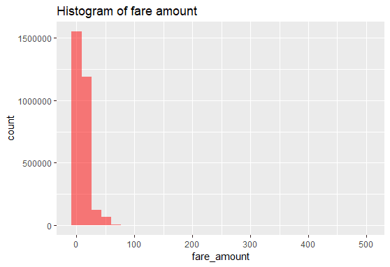
資料整理後,EDA開始
1. Fare_Amount
平均值為11.33
分布也主要集中在2.5~12.5之間
 2. Year and Fare
年與年之間沒有太大差別

3. Month and Fare
月與月間一樣沒特別差異
我畫的圖好漂亮~

4. Day and Fare
禮拜幾一樣沒特別差異

Training 的RMSE表現得比 Cross validation set還好,正常現象,
看起來nrounds還可以繼續再跑更深,不過電腦已經跑半小了,所以我選擇先打住
而best rounds = 300

1. Minkowski Distance: 曼哈頓距離與歐幾里得距離
先把函數寫好:
minkowski_distance <- function(x1, x2, y1, y2, p) {
  return ((abs(x2 - x1)^p) + (abs(y2 - y1))^p)^(1 / p)
}
2. 把pick up datetime的時間分解出來變成年 / 月 / 日 / 時
3. 同時將禮拜一到日的變數抓出來(dayofweek);時刻也抓出來(hour)
4. 將hour再進行一次特徵工程,分為Morning / Mid-Day / Evening / Night
5. 用經緯度取出經緯度的差距
6. 曼哈頓距離
#Feature engineering I, time & distance

full<-full%>%
  mutate(
    pickup_datetime = ymd_hms(pickup_datetime), #split time
    year = as.factor(year(pickup_datetime)),
    month = as.factor(month(pickup_datetime)),
    day = as.numeric(day(pickup_datetime)),
    dayofweek = as.factor(wday(pickup_datetime)), #Monday to Sunday
    hour = as.numeric(hour(pickup_datetime)),
    timeofday = as.factor(ifelse(hour >= 3 & hour < 9,
                                 "Morning", ifelse(hour >= 9 & hour < 14, "Mid-Day",
                                                   ifelse(hour >= 14 & hour < 18, "Evening", "Night")))),
    lat_diff=abs(dropoff_latitude)-abs(pickup_latitude),
    long_diff=abs(dropoff_longitude)-abs(pickup_longitude),
    manhattan=minkowski_distance(pickup_longitude,dropoff_longitude,pickup_latitude,dropoff_latitude,1),
  ) %>%
  select(-pickup_datetime)
7. 半正矢公式: 地球是圓的,自然需要特殊的方法求出真正的地理距離,而半正矢公式便是藉由經緯度來確認大圓上兩點的距離的方法,R語言裡有distHaversine函數可以計算
full<-full%>%
  mutate(dist = distHaversine(cbind(pickup_longitude, pickup_latitude), cbind(dropoff_longitude, dropoff_latitude),
                              r = 6371))
#地球半徑為6371 KM
我們發現有pickup 與 drop off 一樣的位子,但卻有徵收費用的情況,初步判斷應該是取消的手續費,因此特別再篩選出來做為cancel變數
full  %>% filter(dist==0)  %>% count(sep)
full  %>% filter(fare_amount!=0) %>%
  filter(dist==0)  %>% count(sep)
full$cancel=ifelse(full$dist==0,1,0)
現在稍微看一下整體的狀況:
head(full)

> head(full)
  fare_amount pickup_longitude pickup_latitude dropoff_longitude dropoff_latitude passenger_count   sep
1         4.5        -73.84431        40.72132         -73.84161         40.71228               1 train
2        16.9        -74.01605        40.71130         -73.97927         40.78200               1 train
3         5.7        -73.98274        40.76127         -73.99124         40.75056               2 train
4         7.7        -73.98713        40.73314         -73.99157         40.75809               1 train
5         5.3        -73.96810        40.76801         -73.95665         40.78376               1 train
6        12.1        -74.00096        40.73163         -73.97289         40.75823               1 train
  year month day dayofweek hour timeofday  lat_diff long_diff manhattan     dist cancel
1 2009     6  15         2   17   Evening -0.009041 -0.002701  0.011742 1.030764      0
2 2010     1   5         3   16   Evening  0.070701 -0.036780  0.107481 8.450134      0
3 2011     8  18         5    0     Night -0.010708  0.008504  0.019212 1.389525      0
4 2012     4  21         7    4   Morning  0.024949  0.004437  0.029386 2.799270      0
5 2010     3   9         3    7   Morning  0.015754 -0.011440  0.027194 1.999157      0
6 2011     1   6         5    9   Mid-Day  0.026603 -0.028072  0.054675 3.787239      0
> head(new)
  fare_amount pickup_longitude pickup_latitude dropoff_longitude dropoff_latitude passenger_count   sep
1         4.5        -73.84431        40.72132         -73.84161         40.71228               1 train
2        16.9        -74.01605        40.71130         -73.97927         40.78200               1 train
3         5.7        -73.98274        40.76127         -73.99124         40.75056               2 train
4         7.7        -73.98713        40.73314         -73.99157         40.75809               1 train
5         5.3        -73.96810        40.76801         -73.95665         40.78376               1 train
6        12.1        -74.00096        40.73163         -73.97289         40.75823               1 train
  year month day dayofweek hour timeofday  lat_diff long_diff manhattan     dist cancel
1 2009     6  15         2   17   Evening -0.009041 -0.002701  0.011742 1.030764      0
2 2010     1   5         3   16   Evening  0.070701 -0.036780  0.107481 8.450134      0
3 2011     8  18         5    0     Night -0.010708  0.008504  0.019212 1.389525      0
4 2012     4  21         7    4   Morning  0.024949  0.004437  0.029386 2.799270      0
5 2010     3   9         3    7   Morning  0.015754 -0.011440  0.027194 1.999157      0
6 2011     1   6         5    9   Mid-Day  0.026603 -0.028072  0.054675 3.787239      0
資料整理後,EDA開始
1. Fare_Amount
平均值為11.33
分布也主要集中在2.5~12.5之間
summary(full$fare_amount)
   Min. 1st Qu.  Median    Mean   3rd Qu.    Max.    NA's
   2.50    6.00    8.50   11.33   12.50    500.00    9914
ggplot(train,aes(x=fare_amount))+
  geom_histogram(fill="red",alpha=0.5) +
  ggtitle("Histogram of fare amount")

ggplot(train,aes(x=log1p(fare_amount)))+
  geom_histogram(fill="red",alpha=0.5,binwidth=0.25)+
  ggtitle("Histogram of log fare_amount")
年與年之間沒有太大差別
full  %>% filter(sep=="train") %>%
  group_by(year) %>%
  summarize(Mfare = mean(fare_amount))
# A tibble: 7 x 2
  year  Mfare
  <fct> <dbl>
1 2009   10.0
2 2010   10.2
3 2011   10.4
4 2012   11.2
5 2013   12.6
6 2014   12.9
7 2015   13.0

3. Month and Fare
月與月間一樣沒特別差異
我畫的圖好漂亮~
  full  %>% filter(sep=="train") %>%
  group_by(month) %>%
  summarize(Mfare = mean(fare_amount))
# A tibble: 12 x 2
   month Mfare
   <fct> <dbl>
 1 1      10.7
 2 2      10.9
 3 3      11.2
 4 4      11.3
 5 5      11.6
 6 6      11.5
 7 7      11.1
 8 8      11.2
 9 9      11.7
10 10     11.6
11 11     11.6
12 12     11.6

4. Day and Fare
禮拜幾一樣沒特別差異
  full %>% filter(sep =="train") %>%
  group_by(dayofweek)%>%
  summarise(mean = mean(fare_amount))
# A tibble: 7 x 2
  dayofweek  mean
  <fct>     <dbl>
1 1          11.6
2 2          11.4
3 3          11.2
4 4          11.3
5 5          11.5
6 6          11.4
7 7          11.0

5. 集群分析
稍微查證了一下紐約市的行政區,一共有五個,所以在此使用Kmean 將其集群為五個群體,為了之後套用Xgboost建模,再one hot encoding一次
colnames(full)
cluster <- full[,2:5]
kcluster <- kmeans(cluster, centers=5)
full$cluster <- kcluster$cluster
full$cluster <- as.factor(full$cluster)

#Make it dummy
DummyTable <- model.matrix( ~ cluster, data = full)
new <- cbind(full , DummyTable[,-1])
head(new)
new <- new[,-19]
Modeling
一樣丟Xgboost
1. 準備好測試與訓練集
2.轉DMatrix格式
3.Cross validation 求出最佳的rounds(同時調一下Early stopping避免訓練過頭)
4. 訓練集建模
5. 預測Testing set
train=new  %>% filter(sep=="train")  %>% select(-sep)
test=new  %>% filter(sep=="test")  % >% select(-sep)
x_train<- model.matrix(~.-1, data = train[,-1])
x_test <- model.matrix(~.-1, data = test[,-1])
train_label=train$fare_amount
test_label=test$fare_amount
xgbtrain = xgb.DMatrix(x_train,label = train_label)
xgbtest = xgb.DMatrix(x_test,label = test_label)

p <- list(objective = "reg:linear",
          eval_metric = "rmse",
          max_depth = 8 ,
          eta = .05, #.05
          subsample=1,
          colsample_bytree=0.8,
          num_boost_round=1000,
          nrounds = 300)


cv.model = xgb.cv(
  params = p,
  data = xgbtrain,
  nfold = 5,
  nrounds=300,
  early_stopping_rounds = 100,
  print_every_n = 20)
Training 的RMSE表現得比 Cross validation set還好,正常現象,
看起來nrounds還可以繼續再跑更深,不過電腦已經跑半小了,所以我選擇先打住
而best rounds = 300
> cv.model
##### xgb.cv 5-folds
    iter train_rmse_mean train_rmse_std test_rmse_mean test_rmse_std
       1       13.888190    0.007455456      13.890179    0.03448709
       2       13.260992    0.005683884      13.264712    0.03583208
       3       12.666969    0.006196342      12.672735    0.03481734
       4       12.106341    0.006029217      12.113125    0.03405810
       5       11.575596    0.006358640      11.584849    0.03310157
---
     296        3.278589    0.005333968       3.712828    0.03897361
     297        3.277584    0.005416254       3.712506    0.03901520
     298        3.276595    0.005302650       3.712396    0.03891970
     299        3.275502    0.005347438       3.712143    0.03882068
     300        3.274536    0.005240955       3.712034    0.03878134
best.nrounds = cv.model$best_iteration
> best.nrounds
[1] 300

xgb.model = xgb.train(paras = p,
                      data = xgbtrain,
                      nrounds = best.nrounds)
來看看最後importance
其實已經可以由剛剛EDA的探索大概能知道,不同時段對於費用的影響其實沒有特別大~~~
xgimportance <- xgb.importance(xgb.model, feature_names = colnames(xgbtrain))
head(xgimportance)

> head(xgimportance)
             Feature       Gain      Cover  Frequency
1:              dist 0.82563276 0.09538532 0.07091163
2: dropoff_longitude 0.04234086 0.14592193 0.13166697
3:  pickup_longitude 0.01909929 0.13338461 0.15964240
4:         long_diff 0.01879777 0.09521342 0.07559448
5:         manhattan 0.01781278 0.04081037 0.07097245
6:  dropoff_latitude 0.01639659 0.11556195 0.10223195
有不少重要因素是特徵工程轉換而來的,而第一名半正矢距離跟第四名曼哈頓距離都是屬於經緯度的轉換,也不意外同為經緯度的變數分別在2 ~4 與第6名,整體而言,距離單位以及地理位置的變數對於計程車費率影響還是大於時間相關的變數,其實已經可以由剛剛EDA的探索大概能知道,不同時段對於費用的影響其實沒有特別大~~~
fare_amount = predict(xgb.model, xgbtest)
#預測
submission <- cbind(key,fare_amount)
write.csv(submission,file = "submission.csv", row.names = F)

繳交後的RMSE為3.07051
個人覺得還不錯,
但心裡仍然覺得有很多地方可以再精進,例如許多Kernel都把紐約市裡著名的地標抓出來並算出pickup 與 drop off 和重要地標的距離作為變數;以及針對passenger amount的處理,0乘客的筆數實際上有不少個,而本次並未對此進行特徵處理,另外對於集群的效果似乎也未達預期,或許可以改成和Kaggle其他作者一樣針對著名地標做處理。
最後對於調參的部分,看起來如果繼續迭代下去,RMSE或許還可以因此再降下來一些,不過硬體設備可能已經到達極限了
這次分析給自己兩週的時間進行,分析的數量到達300萬筆,這樣透過程式語言進行修改分析的感覺真的蠻暢快的,要進步要開眼界果然還是要自己主動去接觸資料及然後分析~~~~
這份資料集還有很多方向可以努力
之後應該會有個Part II
繼續努力!!!!


留言
張貼留言